Features
What you can actually do with it
PVDCal is a unit-cell solver: one drain, the soil cylinder it serves, and everything below resolved inside it. Every screen here is the application itself, not an illustration, and underlined terms carry a plain-English note.
Input
Your profile, layer by layer
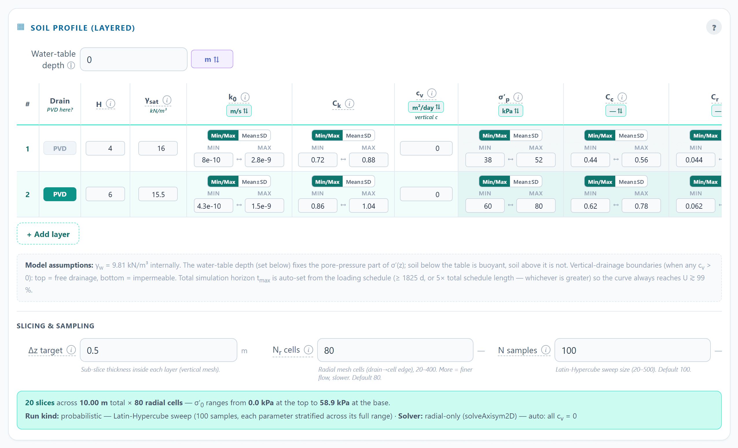
A layered soil table carries what a consolidation calculation actually needs, and the tool derives the rest in front of you.
- Compression and recompression indices, preconsolidation pressure, void ratio, unit weight and permeability per layer.
- Permeability that follows effective stress through the permeability change index, rather than staying fixed.
- Undrained modulus for the immediate settlement as the embankment is placed.
- Water table depth, with the in-situ effective stress profile computed and plotted.
Soil model
A smooth transition through yielding
The classical method switches from recompression to virgin compression the instant effective stress crosses σ′p. That is a modelling convenience, not an observation.
- Real clays do not yield at a single pressure: a natural deposit holds a spread of particle arrangements, bond strengths and stress histories, and they do not all give way at once.
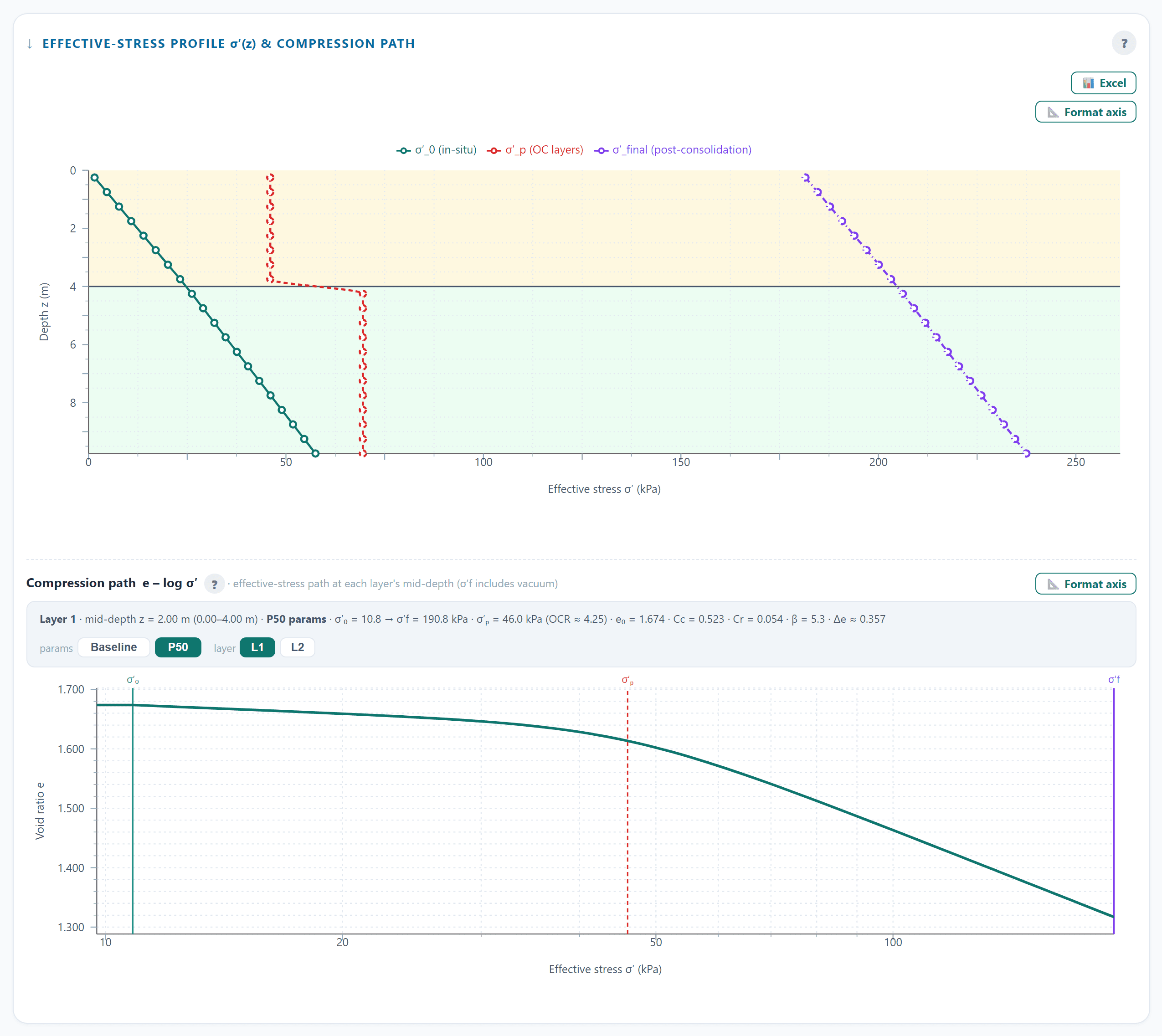
- PVDCal blends the compression index across the yielding zone instead of stepping it, which is both the more honest description and the better-behaved one numerically.
- Settlement is integrated in small effective-stress increments, each evaluated at the geometric mean of its own end points.
- The width of the transition is yours to set, and the compression path is drawn so you can see exactly where the layer yields.
Drains
Band drains as installed
Geometry, pattern and the disturbance around the mandrel are all inputs, not assumptions.
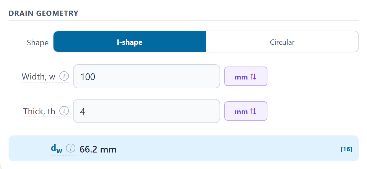
- Band (I-shape) or circular drains, converted to an equivalent diameter.
- Square or triangular patterns, with the radius of influence and the drains per hectare each implies.
- Smear and transition zones with their own permeability ratios.
- Well resistance checked against the discharge capacity you specify.
Partial penetration
Drains that stop short of the base
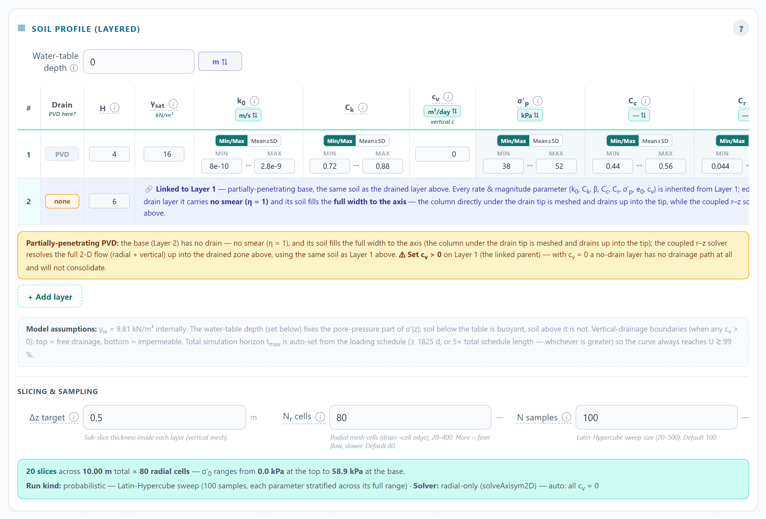
Drains are not always taken to the bottom of the compressible profile — because of rig reach, cost, or a layer nobody wants to puncture. PVDCal models that case as it is, rather than pretending the drain runs full depth.
- Mark any layer as having no drain: the treated depth drains radially to the drain, while the untreated layer below keeps draining vertically to whatever boundary it has.
- Below the drain tip the mesh switches to a full disk to the axis, so flow around and under the tip is resolved instead of assumed.
- Splitting a layer at the drain tip is offered as a decision, not done silently, and the split inherits the parent layer's parameters.
- The case is verified at its limits: a drain through the full depth reproduces the classical radial solution, and no drain at all reproduces vertical consolidation.
Loading
Construction as it is built
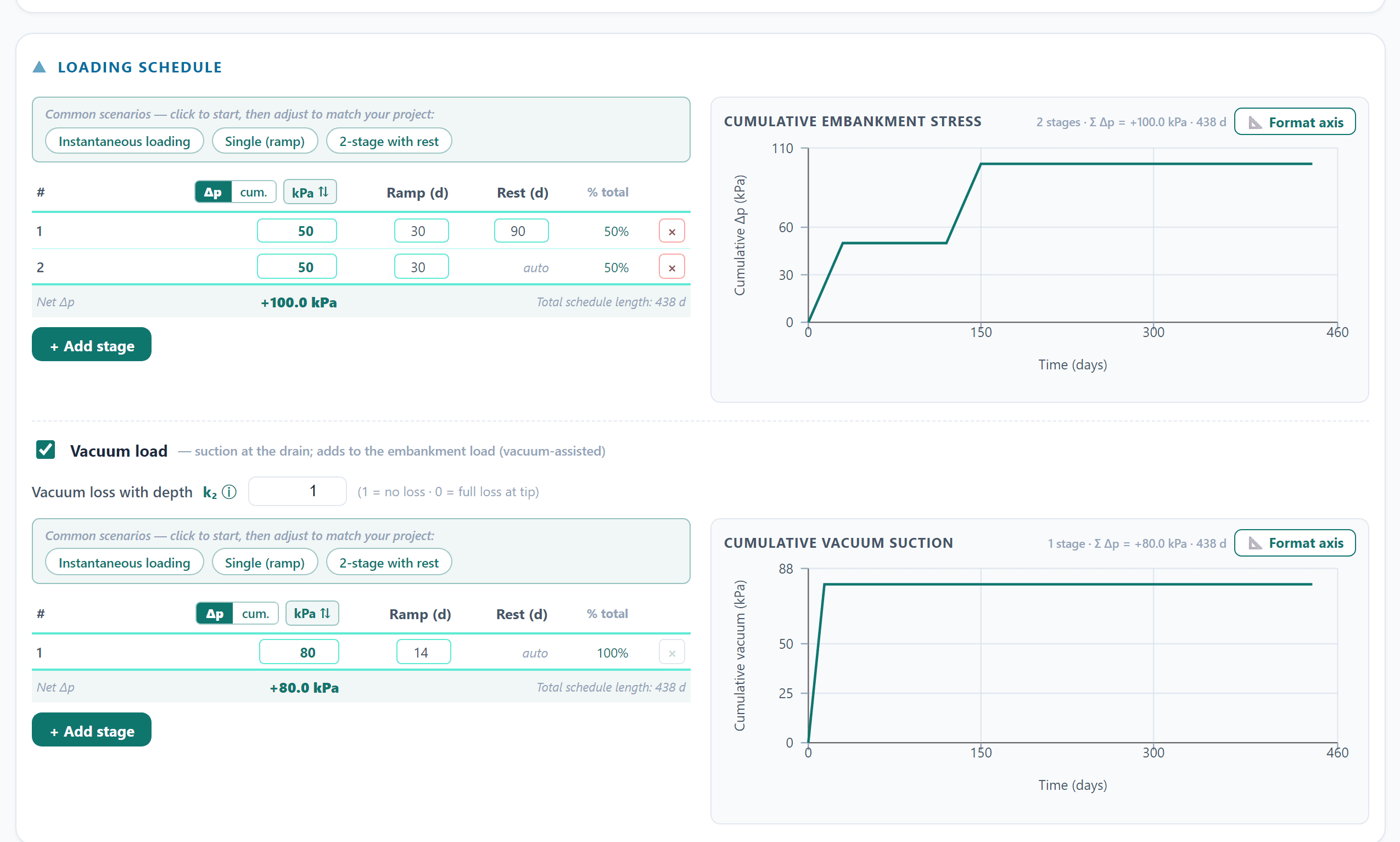
Fill goes on in stages, with rest periods, and sometimes vacuum does part of the work.
- Multi-stage ramp loading with rest periods and surcharge removal.
- Vacuum preloading as a suction boundary on the drain, including loss with depth.
- Unload and reload along a recompression path, so removing surcharge is not treated as virgin compression.
- Creep carried through the run, so long programmes are not flattered.
Probabilistic design
Ranges in, bands out
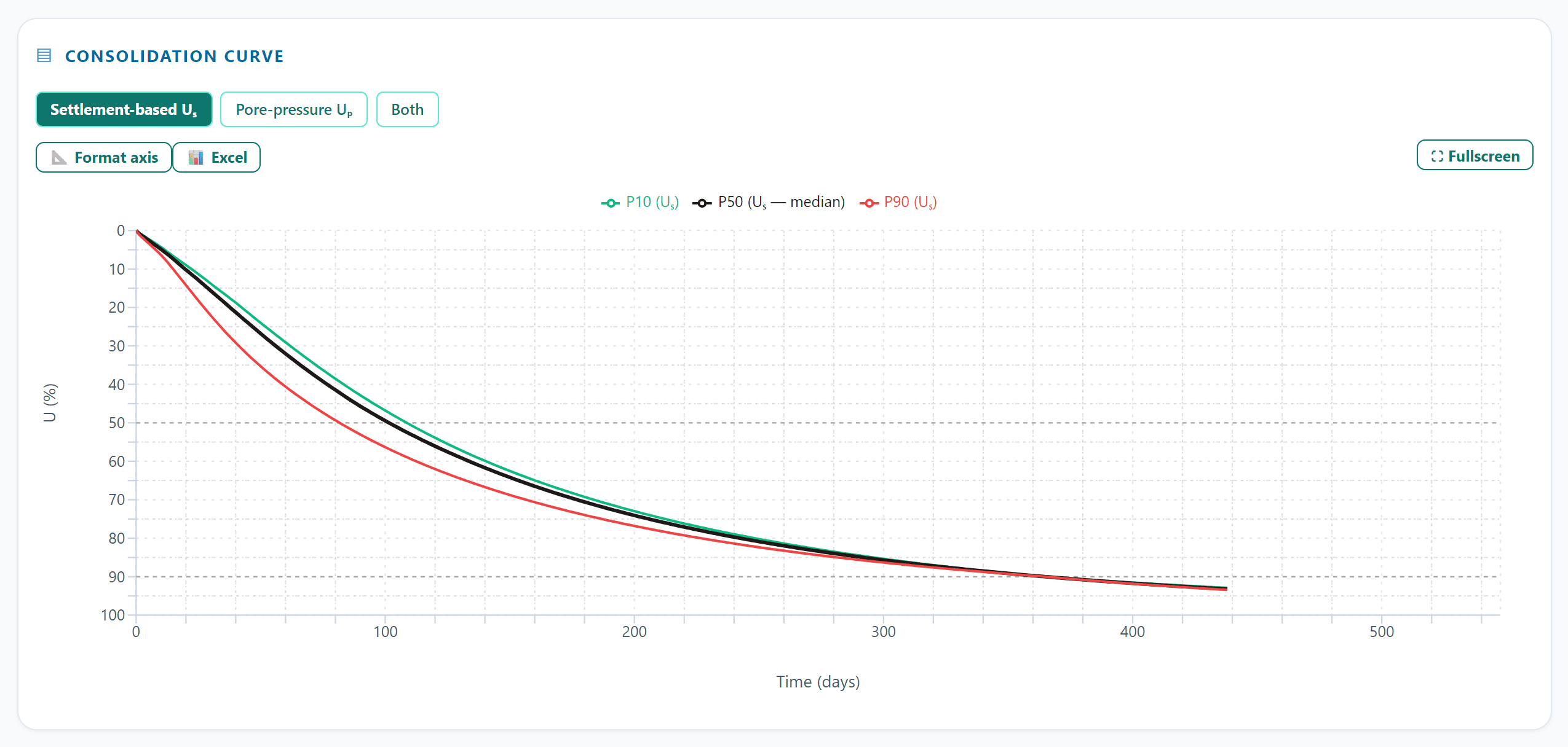
Give any input as a range and every sample runs a complete spacing search, so the band is a band of answers, not of inputs.
- Latin-Hypercube sampling across the ranges you set.
- P10, P50 and P90 spacing for both patterns, with the drains per hectare each implies.
- A sensitivity card ranking which input moved the answer most.
- Runs spread over parallel workers, with results identical to a single-threaded run.
Results
Everything the calculation knows
Results open as cards you can read, format and export — not a single printout.
- Consolidation and settlement against time, settlement-based or pore-pressure-based.
- Effective stress with depth, and the compression path per layer.
- Settlement plates and pore-pressure probes at any depth you choose.
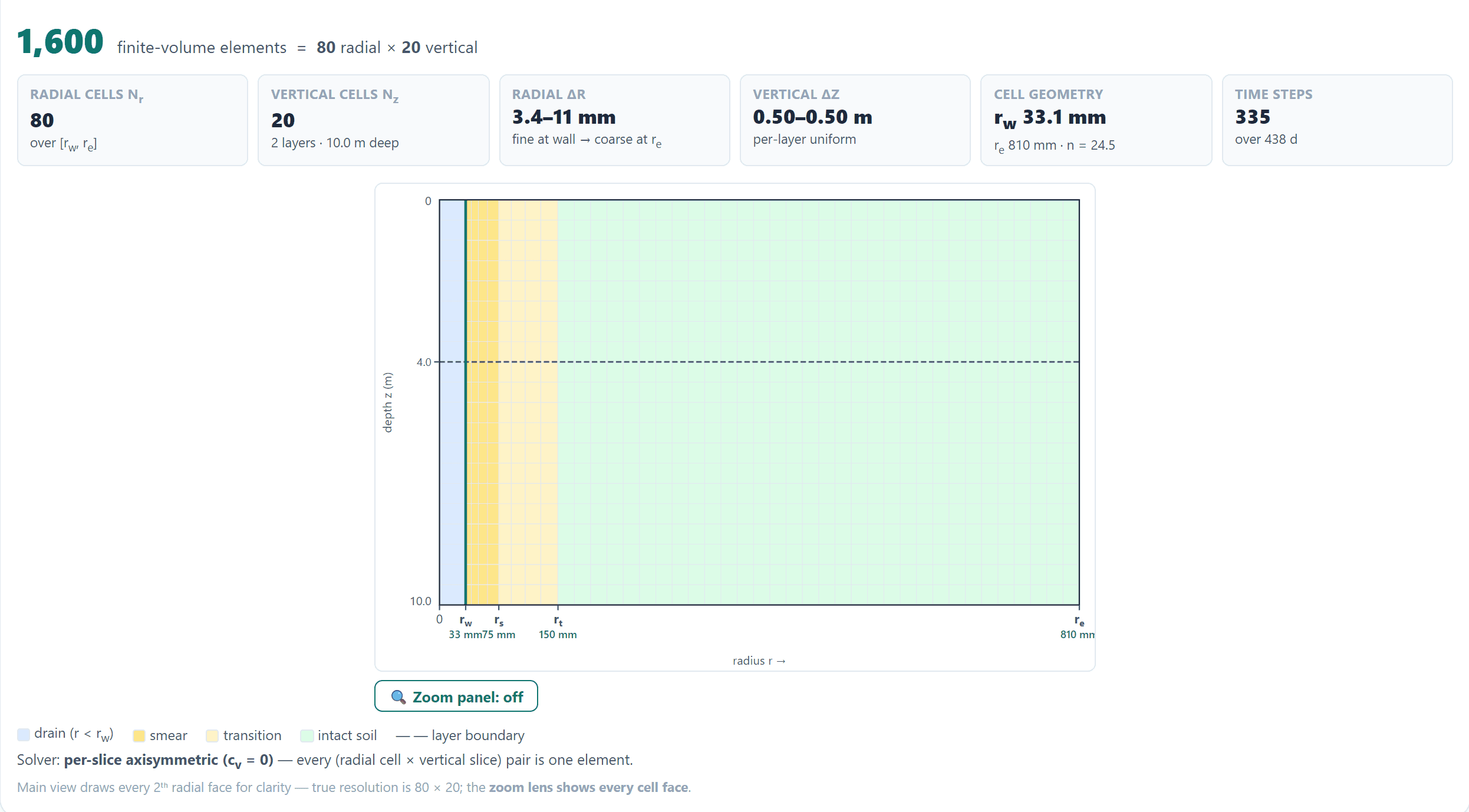
- The numerical mesh itself, with a zoom lens over the cells near the drain.
- Excel export from any chart, and image or animation export for reports.
Heat map
Watch the pore pressure leave the ground
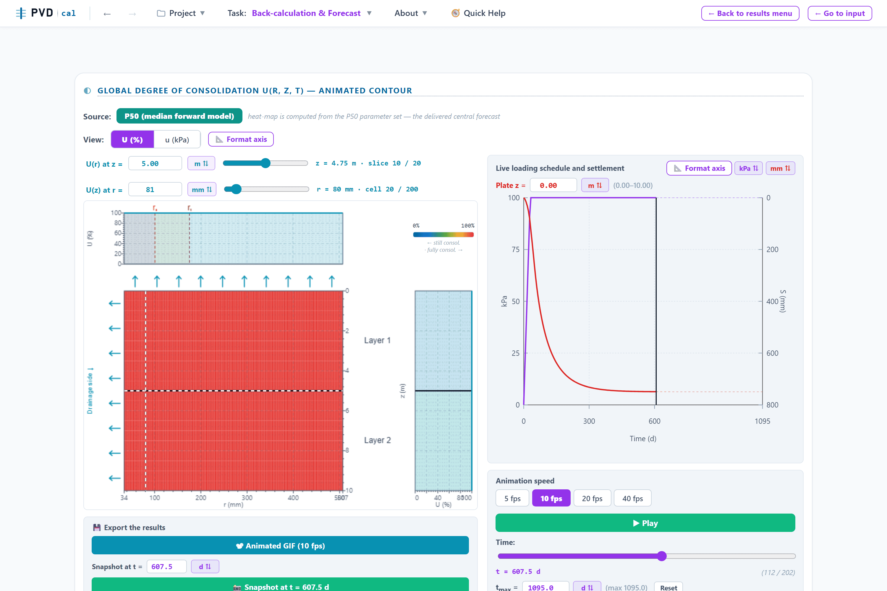
An animated heat map of consolidation across the unit cell, so the calculation stops being a number and becomes something you can see.
- Play it through the programme, or drag the time slider to any day and read the state of the ground at that moment.
- Switch between degree of consolidation and excess pore pressure in kPa, with the smear and transition boundaries marked on the radius axis.
- Slice it: a profile with depth at a chosen radius, and a profile with radius at a chosen depth, both moving with the animation.
- Export an animated GIF for a report or a presentation, or a snapshot at one instant — the loading schedule and settlement play alongside, so cause and effect sit on the same screen.
Back-analysis
Calibrate against the field, then forecast
Once monitoring starts, the same physics runs backwards: which ground would have produced this record?
- Settlement plates and piezometers used together, in their own units.
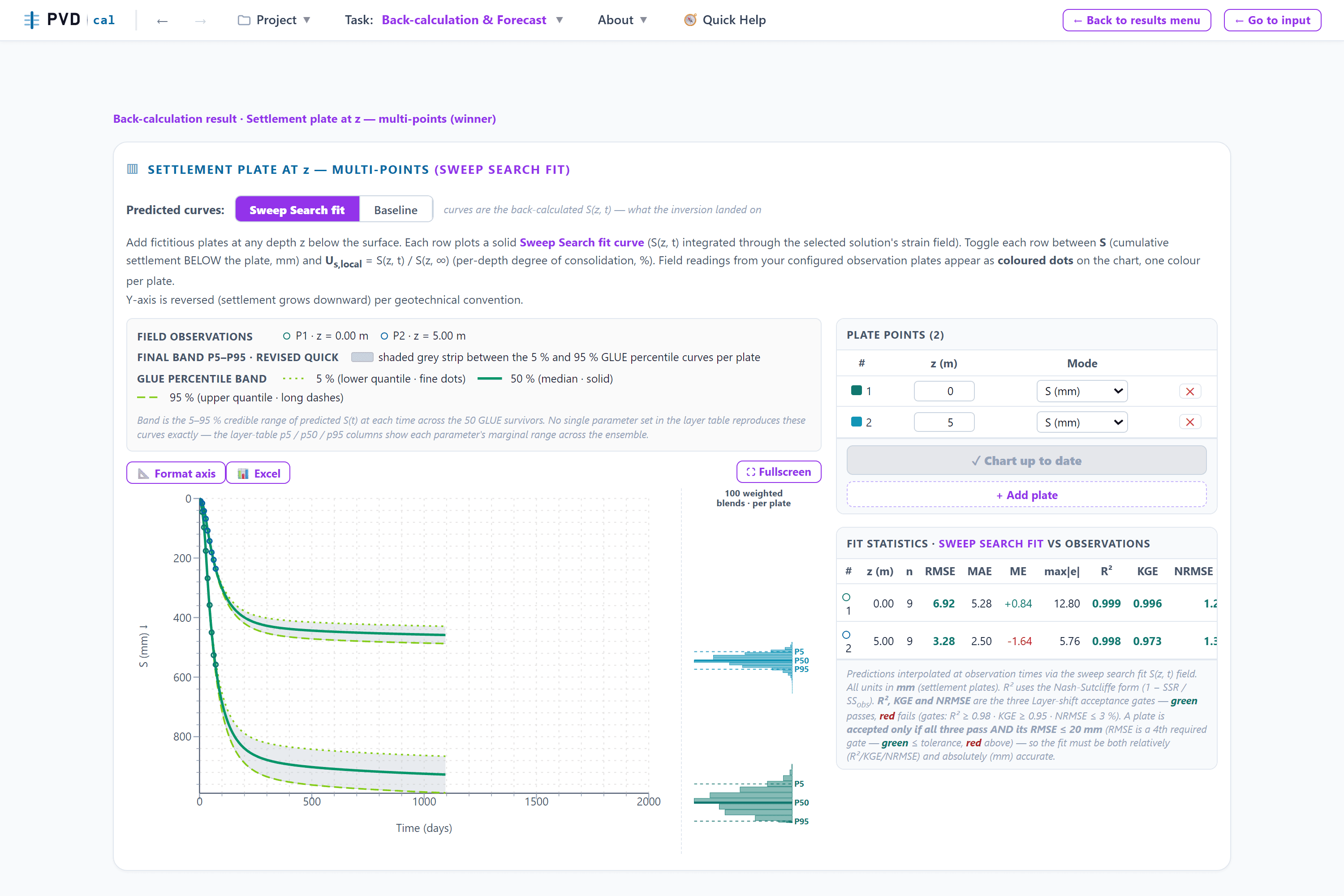
- Sweep Search over permeability, compressibility and rate, within the walls you set — minutes in a browser, where a blind random ensemble of the same family takes hours to days.
- Fit statistics, the parameters recovered, and a flag when a value sits on a bound.
- A forecast range for the settlement still to come, and a cross-check against the Asaoka construction.
Office or site
It runs where the decision is made
There is nothing to install and no licence server to find on a laptop. PVDCal opens in a browser, so the same tool is available at your desk, in the site office, or on the embankment with the plates in front of you.
Laptop, tablet or phone
The full layout — soil tables, observation grids, result cards and charts — has been run on a large-screen phone. More screen means less scrolling, so a tablet or an unfolded phone gives the most comfortable fit in the field.
A report before you leave site
Back-analysis prints a complete report — method, run statistics, the back-calculated profile, the fits against every plate, and the conclusions — straight to PDF from the browser, ready to send from the crest.
Minutes, not an overnight job
The built-in back-analysis example, run on that phone, finished in about twenty minutes — a calibrated fit and a forecast band while the question is still live. An internet connection is needed while you work.
How the solver works, and how it was checked, is set out on the method and validation page.
Try it on your own profile
Start a 7-day free trial. Load an example project, change the soil to yours, and see the spacing band in minutes.