Method and validation
What is solved, and how it was checked
PVDCal does not interpolate a design chart. It solves the governing consolidation equation on a mesh, and every claim on this page is measured by the shipping build.
- 8
- closed-form benchmarks, runnable inside the app
- ≤ 0.53 pp
- mean absolute error on all of them
- 0
- difference between parallel and single-threaded results
- 77–79 %
- of design ranges contained the true settlement in the validation campaign
The numerics
Finite volume on a zone-aware mesh
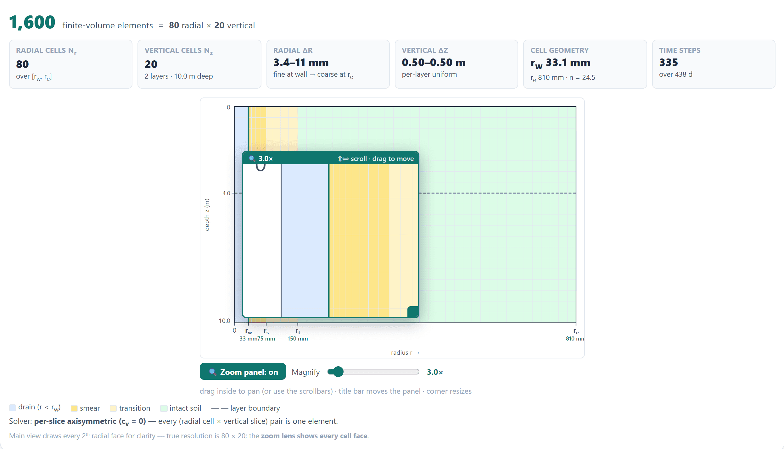
The unit cell around one drain is discretised in radius and depth, and the equation is integrated in time.
- Cell-centred finite volume
- One flux per face, with the permeability taken as the harmonic mean across it. Mass is conserved cell by cell rather than approximately.
- A mesh that knows its zones
- Faces land exactly on the smear and transition boundaries, and on layer interfaces. Cells are fine at the drain and graded coarser into the far field.
- Crank–Nicolson and ADI
- Second-order time stepping in the one-dimensional kernel, and Peaceman–Rachford alternating directions where radial and vertical flow are coupled.
- Coefficients that move
- Permeability and compressibility follow effective stress as consolidation proceeds, which is exactly what the closed-form solutions cannot do.
Scope
What is solved: one drain and its unit cell
PVDCal is a unit-cell solver. It takes the soil cylinder served by a single drain, with no flow across its outer wall, and resolves consolidation across radius and depth inside it. Everything else on this site follows from that.
What that buys you
- Layers, smear, transition zones and a partially penetrating drain are all resolved inside the cell, instead of being averaged into one coefficient.
- A design run is seconds of computation, so a whole probabilistic sweep is minutes rather than an overnight job.
- It is the same idealisation the classical design charts rest on, so results can be checked directly against them.
What it assumes, and where that bites
- Every drain is identical and equally loaded, so the outer wall carries no flow. Real drain fields are not perfectly regular.
- The rate is therefore over-predicted at block edges, where spacing changes, and next to untreated ground.
- Strains are small: the mesh does not deform as settlement proceeds, which matters where thickness and spacing change materially.
- Lateral spreading, stability and three-dimensional effects are outside it. Use a continuum model where those govern.
Where it fits
A companion to the software you already use
A drain project passes through several kinds of package, and each does its own job well. PVDCal is built to sit beside them, not to replace any of them. No package is named here on purpose: this is a division of labour, not a criticism.
| Tool family | What it does well | What PVDCal adds beside it |
|---|---|---|
| Three-dimensional settlement and consolidation packages | Settlement of arbitrary load layouts at any point, staged construction, and the wider site questions. Drain zones are handled with the classical radial solution and a smear factor. | The drain system itself in finer physics: resolved smear and transition zones, stress-dependent permeability inside the radial field, a smooth yield transition, and vacuum with depth attenuation — plus a Design mode that finds the spacing instead of checking one, and returns it as a band. |
| General-purpose finite-element suites | The peripheral geometry: differential settlement, stability, soil–structure interaction, with drains as line elements or explicit meshes. | A unit-cell answer in minutes for screening and design iteration, and calibrated parameters from the monitoring record to feed the larger model — the integration that matters most. |
| One-dimensional settlement tools in national practice | Staged embankment settlement with creep and drain schedules; some fit the computed curve to a settlement-plate record. | Inversion rather than curve scaling: physical layer parameters recovered from every plate and piezometer at once, and a forecast range whose reliability was measured against known truths. |
| Observational constructions kept in spreadsheets | A model-free reading of the trend of the record. | The same construction built in as a cross-check, beside a forecast that carries the physics and states its uncertainty. |
The integration runs through parameters and files, not plug-ins
Calibrate here, model anywhere
Back-analysis returns the layer parameters other packages take as input — permeability, compression indices, the preconsolidation profile, the creep ratio, the smear description — so your own model can be re-run on values the ground has supported rather than the laboratory's first estimate.
Check a design from anywhere
Where the classical assumptions hold, this solver reproduces the analytical radial solution to within one per cent, so a design made elsewhere can be restated here — and the finer physics and the band then show what would change.
Read the record beside any model
Observations import from CSV or Excel, results export the same way, and the whole project travels as a single file you can attach to an email.
The claim is deliberately narrow. Outside the treated area — differential settlement across a footprint, stability, structures — those packages remain the right tools. Inside the unit cell, and from the day the first plate reports, PVDCal does work the general packages do not set out to do.
Verification
Measured against eight closed-form solutions
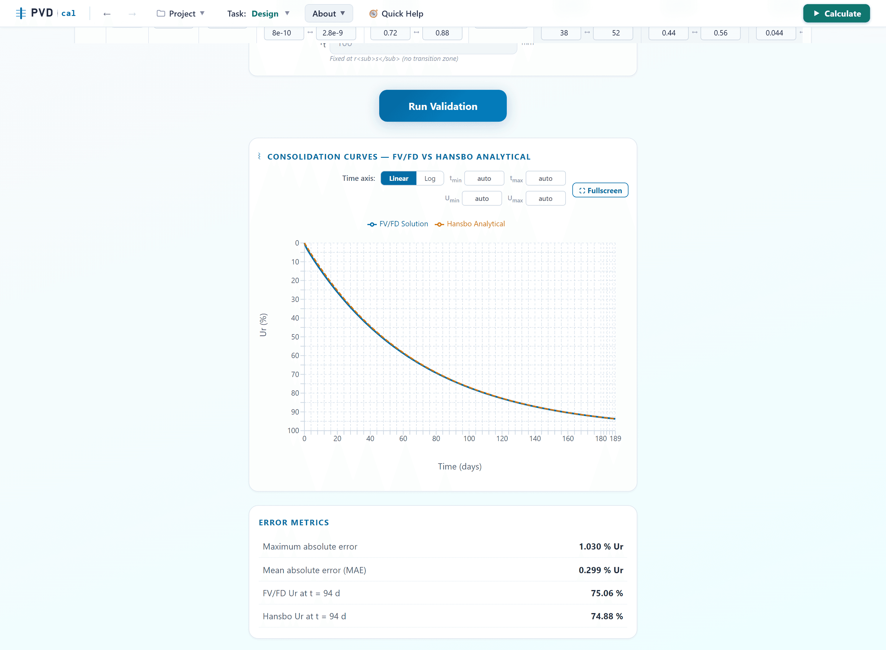
Each benchmark runs from inside the application, so you can repeat these numbers yourself rather than take them from a brochure. Errors are in percentage points of the degree of consolidation.
| Benchmark | What it tests | Mean error | Largest error |
|---|---|---|---|
| Olson–Barron | Ramp loading, ideal drain | 0.398 % | 0.742 % |
| Hansbo | Radial consolidation with smear | 0.299 % | 1.030 % |
| Hansbo, layered solver | Layered stack, ideal drain | 0.530 % | 2.179 % |
| Hansbo with smear, layered solver | Layered stack, with smear | 0.254 % | 0.963 % |
| Terzaghi | Pure vertical drainage | 0.116 % | 1.119 % |
| Carrillo | Radial and vertical combined | 0.000 % | 0.001 % |
| Vacuum-assisted | Suction boundary condition | 0.530 % | 2.178 % |
| Partial penetration | Limits: full ≡ Hansbo, none ≡ Terzaghi | 0.016 % | 0.290 % |
The larger maximum errors on the two layered radial cases are a single point on the steep initial rise, where the output is sampled most coarsely; they decay immediately afterwards.
What a benchmark can and cannot prove
Each closed-form solution holds only under its own assumptions: constant coefficients, one layer, instantaneous loading. Matching them verifies the machinery — the discretisation, the mesh, the boundary conditions, the time integration.
It cannot verify the extensions beyond them, because no closed form exists for stress-dependent permeability, creep or hysteresis. Those are checked by internal consistency and by degenerate limits: switch the feature off and the classical answer must come back. The real test of the physics is the field comparison below.
Back-analysis method
Sweep Search: an engineered search, then a quasi-Bayesian band
Calibrating soil from a monitoring record is hard because many different soils fit an early record equally well. The usual answers are either one best fit, which hides that problem, or a large random ensemble, which exposes it but costs hours to days of computing.
How it works
The laboratory values you type become walls around the search, widened threefold so a range typed too narrowly cannot fence the truth out. Inside those walls a deterministic grid of three knobs — magnitude, rate and a global speed axis — is swept, with line searches refining between sweeps. Nothing is sampled at random.
The band is then formed by weighting every admissible recipe by its own score: the typed windows act as the prior, the score as the likelihood, and the weighted percentiles approximate the forecast — a quasi-Bayesian propagation step with its reliability measured rather than assumed.
Why it is quick enough to act on
- Minutes in a browser, on a pool of parallel workers, where a blind ensemble of the same family typically needs 10⁴ or more runs and hours to days.
- Planned, not lucky. On the guide's worked toy problem, random draws need about 6000 blind solves to collect 30 useful ones; the planned sweep needs roughly 170.
- Same inputs, same answer, always — so a checker can reproduce your result. Random-ensemble methods differ on every re-run.
- No analyst-chosen threshold. Nothing is accepted or rejected by a cut-off you pick; intervals close on a fixed statistical rule, the same for everyone.
What is claimed, precisely: the speed–magnitude trade-off itself is the well-known rate–compressibility coupling, not a discovery. The specific contribution is carrying a bounded global speed axis through the scan so the magnitude result survives a mis-anchored drainage rate — a measurable design choice, tested in Chapter 30 of the guide, not a general claim of superior accuracy.
Parallel runs
Faster, and identical
Probabilistic runs and back-analysis searches spread their solves across a pool of browser workers. The workers do not carry their own copy of the solver: they take the engine source verbatim at run time, so the arithmetic is the same code.
The workers only solve; the main thread does all the judging, so the answer cannot depend on which worker finished first. An end-to-end parity check runs the same cases through both paths: the current build reports a maximum difference of exactly zero on settlements, pressures and plotted curves.
Validation
Tested against ground whose answer is known
Verification asks whether the equations are solved correctly. Validation asks whether the answers match reality. Both are reported in full in the user guide, including the results that are unflattering.
Synthetic sites, truth withheld
Hundreds of synthetic sites were built from known soils spanning shallow estuarine clay to a 30 m peat–clay stack, with vacuum and partially penetrating cases included. Each site's noisy, cut-short record and a deliberately wrong set of typed parameters were handed to the shipped pipeline. Only after it committed to its ranges was the truth revealed and the hit or miss counted. The design range contained the true final settlement in 77 to 79 % of cases, and the acceptance criteria were registered before the runs.
A monitored embankment
Against a three-metre embankment on PVD-improved marine clay, monitored for about three years, the tool was given the record up to a cut day and asked to forecast the rest. From a 400-day record the forecast was 1.5 % away from the final settlement, and from a 700-day record 0.8 %. From a 200-day record it was 9.4 % out and its range missed: back-analysis earns its place only once the record is long enough, and the guide says so.
The full method, every benchmark, the convergence study and the campaign are documented in the user guide, which is free to download.
See it on your own profile
Start a 7-day free trial. Load an example project, change the soil to yours, and see the spacing band in minutes.