Worked example
From soil profile to surcharge removal
This is the path a drain project takes through PVDCal. Every project in the app can be loaded as a ready-made example, so you can reproduce each step rather than read about it.
STEP 01
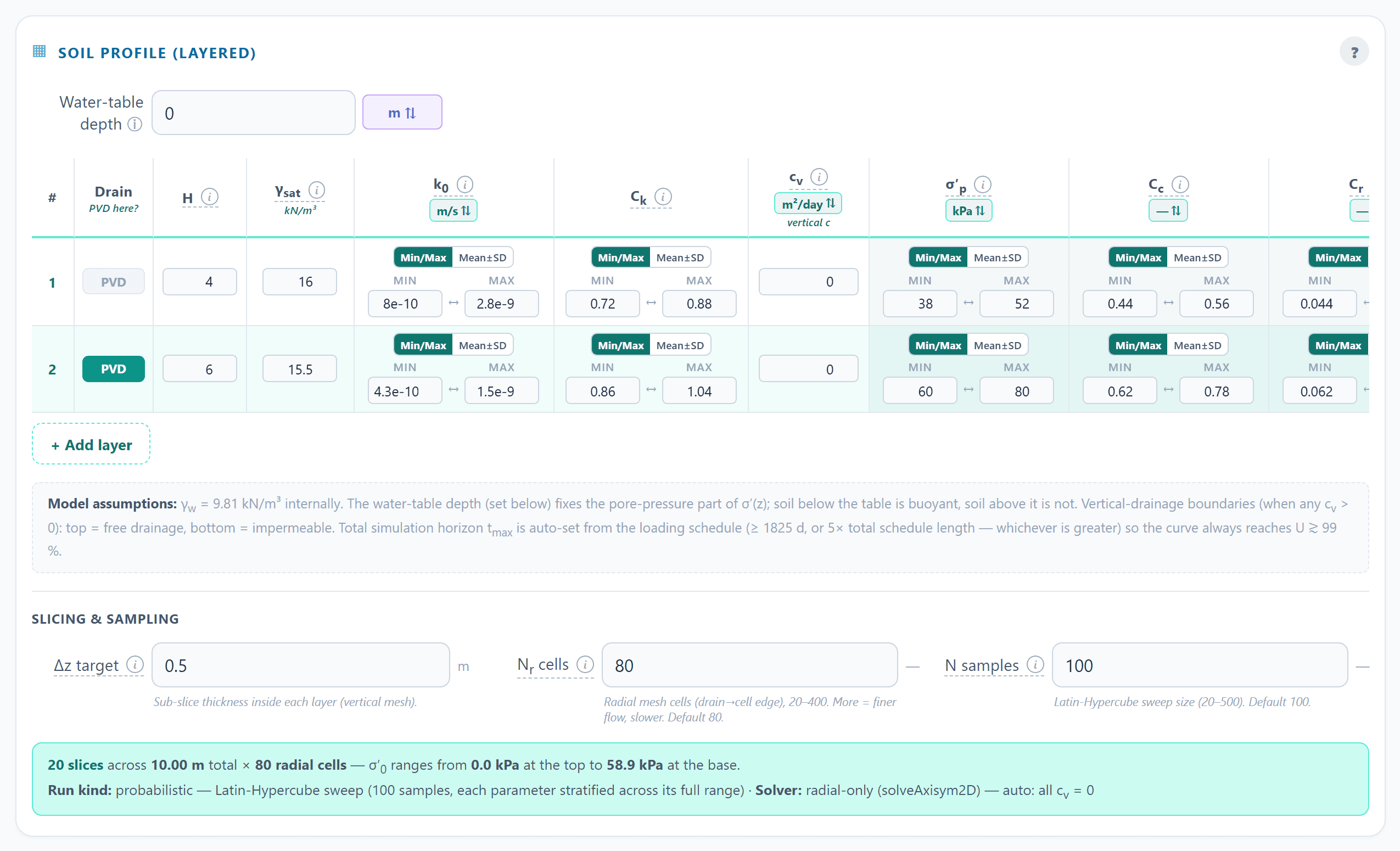
Describe the ground
A two-layer soft-clay profile goes in with its compression indices, preconsolidation pressures and permeabilities. Where a parameter is uncertain, a low and a high value are given instead of one number. The water table sets the in-situ effective stress profile.
STEP 02
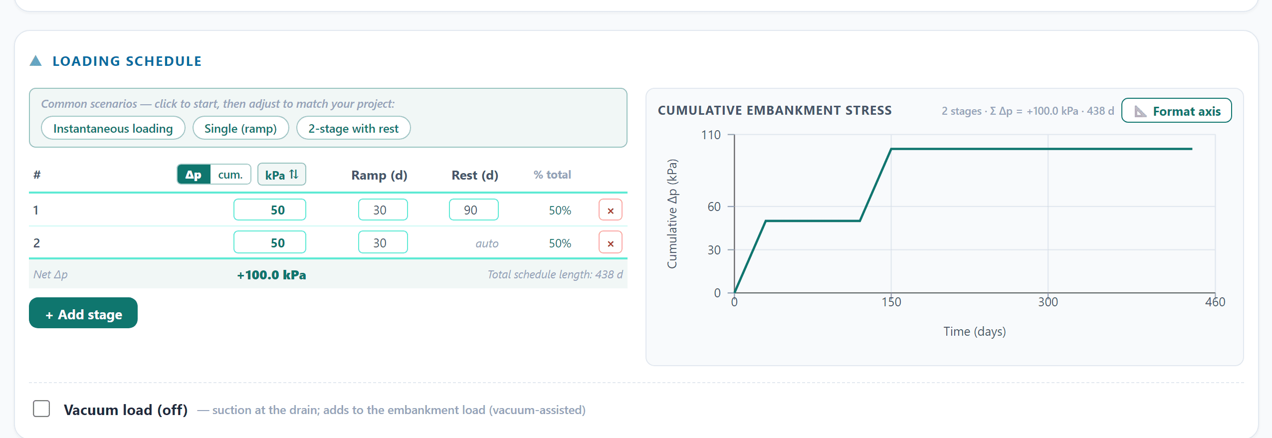
State the target and the construction
Ninety per cent consolidation within a year, under fill placed in two stages with a rest period. Vacuum can be added here, and drains can be told to stop above the base of the profile.
STEP 03
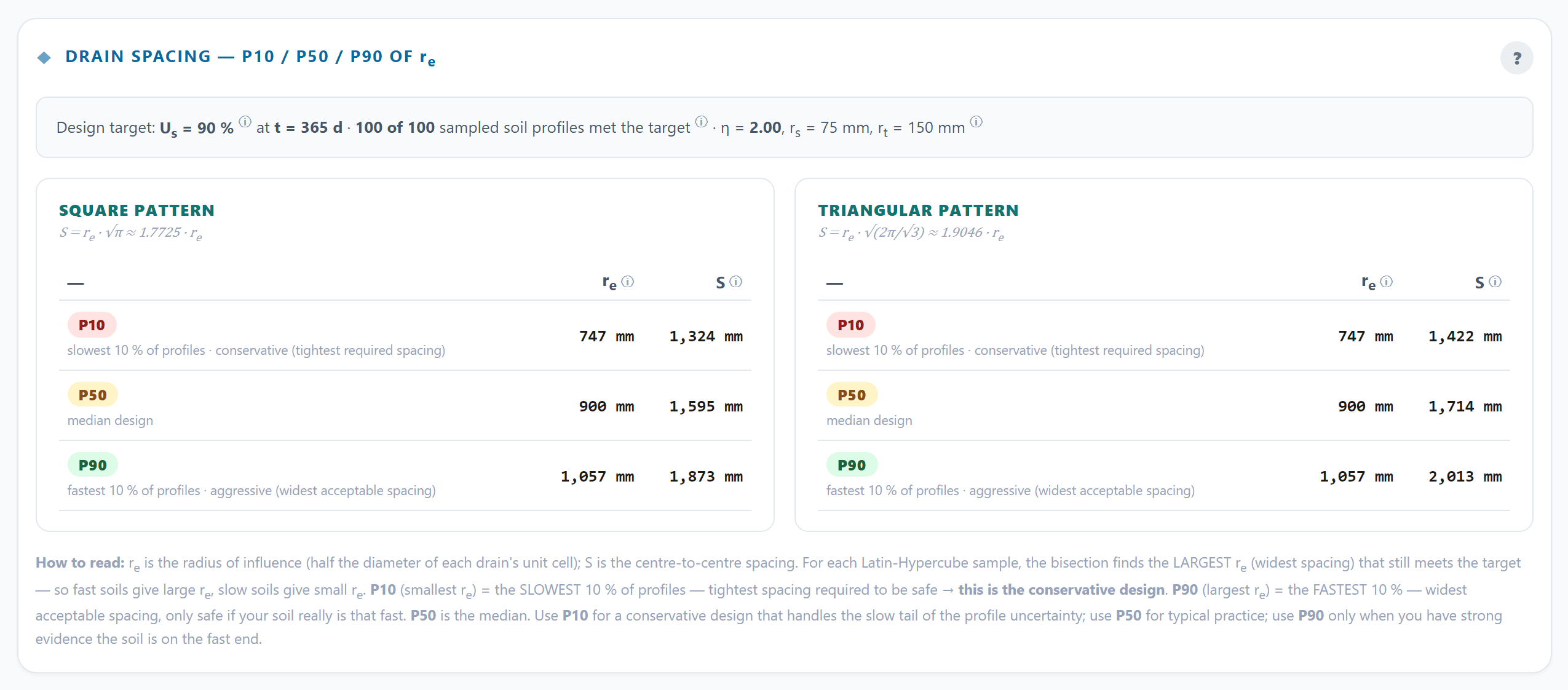
Get a spacing band, not a single number
Each sample of the uncertain parameters runs its own complete spacing search, so the result is the spread of answers the ground allows: the P10, P50 and P90 spacing for square and triangular patterns, and the drains per hectare each implies.
STEP 04
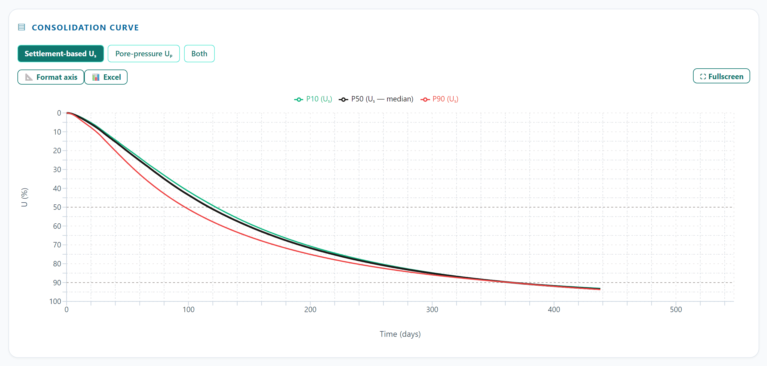
Check what the answer depends on
The consolidation curve shows how the ground gets there, and a sensitivity ranking shows which input actually moved the spacing. That is where another borehole or laboratory test is worth its cost.
STEP 05
Once built, let the ground correct you
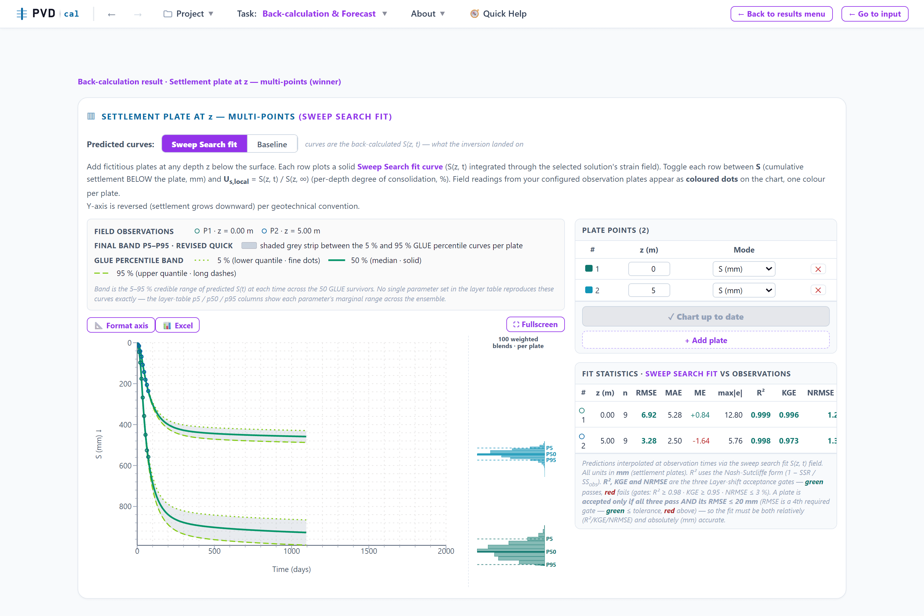
Settlement plates and piezometers go in as they are read. The search finds the ground that explains the record, reports how well it fits, and forecasts what is still to come with a credible range — the number that decides when surcharge comes off.
Does it work?
Two results from the user guide
Both are reported in full there, with the method used to score them.
A site whose truth was known
On a test site built from a hidden soil, the typed laboratory values alone drifted to a final settlement 13 % too high. Given only the noisy record up to the halfway point, the calibrated answer tracked the hidden truth beyond the cut, and the design range of 991 to 1168 mm bracketed the true 1113 mm.
A real embankment
On a monitored embankment on marine clay, forecasts made from 400-day and 700-day records came within 1.5 % and 0.8 % of the final measured settlement. From a 200-day record the error was 9.4 % and the range missed — the record was simply too short, and the guide reports that alongside the successes.
The method behind these numbers is on the method and validation page.
Run this example yourself
Start a free trial, open Example projects, and press Calculate. The run you get is the one on this page.